If you have spent any time in the world of project risk management, you have likely run into two heavyweight contenders. In one corner, we have the reliable, straightforward Triangular distribution. In the other, the sophisticated, smooth-curved Beta (or PERT) distribution.
Choosing between them can feel like a philosophical debate. Do you prefer the ‘safety’ of straight lines, or the ‘realism’ of a bell curve? It might seem like a small detail, but as we will see today, the choice you make can shift your P90 deadline by days or even weeks.
Today, we are going to put these two models head-to-head. We will look at the math (no PhD required), run a Python simulation to see how they behave, and ultimately help you decide which one deserves a spot in your next project report.
The Straight-Shooter: The Triangular Distribution
As we discussed in our last article, the Triangular distribution is the ‘simplest’ way to model uncertainty. You provide an Optimistic (A), a Most Likely (M), and a Pessimistic (B) value. The computer draws a literal triangle between those points.
The math for the average (the mean) is dead simple:
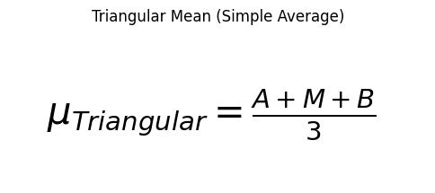
Because it uses straight lines, the Triangular distribution gives significant ‘weight’ to the areas between your points. It assumes that as you move away from your ‘Most Likely’ value, the probability drops off at a steady, linear rate. It doesn’t ‘judge’ your estimates; it simply connects the dots.
The Sophisticate: The Beta (PERT) Distribution
The Beta distribution (often called the PERT distribution in project management) is a bit more refined. Instead of a jagged triangle, it produces a smooth, bell-shaped curve.
The biggest difference lies in how it treats your ‘Most Likely’ (M) estimate. The Beta distribution assumes that your expert’s most likely guess is much more powerful than the extremes. In fact, the standard PERT formula gives the Most Likely value four times the weight of the Optimistic or Pessimistic values:
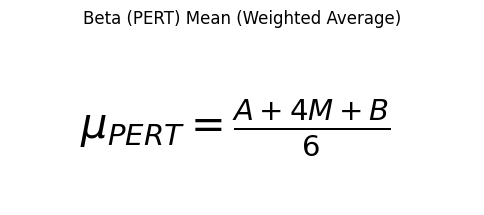
Notice the denominator is 6. We are essentially taking six ‘votes’: one for A, four for M, and one for B. This ‘pulls’ the average much closer to the center and makes the ‘tails’ of the distribution much thinner.
Head-to-Head: The ‘Conservative’ Gap
Why does this matter to you? It comes down to risk appetite.
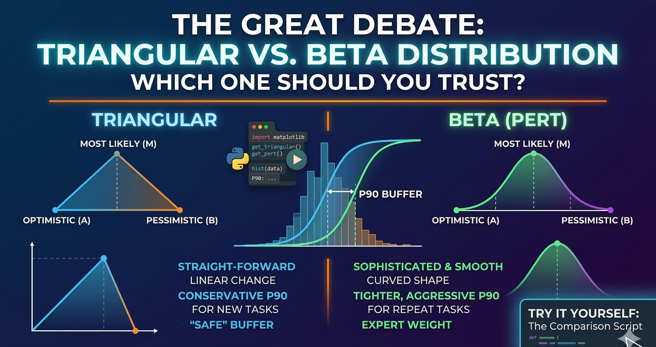
Because the Triangular distribution has ‘fatter’ tails, it assumes there is a higher chance of things going moderately wrong. The Beta distribution, however, assumes that extreme outliers—those ‘black swan’ events—are incredibly rare.
If you use the same A, M, and B values for both:
- Triangular will almost always give you a higher, more conservative P90.
- Beta (PERT) will almost always give you a tighter, more ‘aggressive’ P90.
If you are a project manager looking for a ‘safe’ buffer to protect your team from the unknown, the Triangular distribution is your best friend. If you are in a highly competitive environment where every day counts and you trust your Most Likely estimate implicitly, Beta might be your weapon of choice.
In the example below, P90 is 45.8 days for triangular distribution and 37.3 days for betta/PERT distribution. Showing that the triangular esitmate more conservative, and PERT more optimistic.
Try It Yourself: The Comparison Script
If you know a little Python, you can see this gap for yourself. Copy and paste the code below into Google Colab or a Jupyter Notebook.
This script runs 10,000 simulations using both methods and plots them on top of each other. You will clearly see how the ‘Shape of Risk’ changes depending on which math you trust.
import random
import matplotlib.pyplot as plt

# --- 1. USER INPUTS ---
# Let's use a task with a long 'pessimistic' tail to see the difference clearly
A = 10   # Optimistic
M = 20   # Most Likely
B = 60   # Pessimistic (A big 'what-if' risk)
iterations = 10000

# --- 2. THE GENERATORS ---

def get_triangular(a, m, b):
    u = random.random()
    fc = (m - a) / (b - a)
    if u < fc:
        return a + (u * (b - a) * (m - a))**0.5
    else:
        return b - ((1 - u) * (b - a) * (b - m))**0.5

def get_pert(a, m, b):
    # PERT uses the Beta distribution logic
    # We calculate the shape parameters (alpha and beta)
    alpha = 1 + 4 * ((m - a) / (b - a))
    beta = 1 + 4 * ((b - m) / (b - a))
    sample = random.betavariate(alpha, beta)
    return a + (sample * (b - a))

# --- 3. RUN SIMULATIONS ---
tri_data = sorted([get_triangular(A, M, B) for _ in range(iterations)])
pert_data = sorted([get_pert(A, M, B) for _ in range(iterations)])

# --- 4. CALCULATE P90 ---
tri_p90 = tri_data[int(iterations * 0.90)]
pert_p90 = pert_data[int(iterations * 0.90)]

# --- 5. VISUALIZATION ---
plt.figure(figsize=(14, 6))

# Histogram Comparison
plt.subplot(1, 2, 1)
plt.hist(tri_data, bins=50, alpha=0.4, label='Triangular', color='blue')
plt.hist(pert_data, bins=50, alpha=0.4, label='Beta (PERT)', color='green')
plt.title('Distribution Shape: Triangular vs Beta')
plt.xlabel('Days')
plt.ylabel('Frequency')
plt.legend()

# S-Curve Comparison
plt.subplot(1, 2, 2)
probs = [i / iterations for i in range(iterations)]
plt.plot(tri_data, probs, label=f'Triangular (P90: {tri_p90:.1f}d)', color='blue', linewidth=2)
plt.plot(pert_data, probs, label=f'Beta (PERT) (P90: {pert_p90:.1f}d)', color='green', linewidth=2)
plt.axhline(0.90, color='red', linestyle='--', alpha=0.6)
plt.title('Risk Comparison (S-Curve)')
plt.xlabel('Days')
plt.ylabel('Cumulative Probability')
plt.grid(alpha=0.3)
plt.legend()

plt.tight_layout()
plt.show()

print(f"The 'Conservative Gap': {tri_p90 - pert_p90:.2f} days")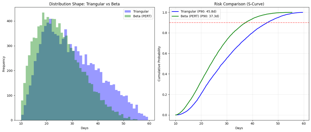
The Verdict: Which one should you use?
There is no ‘wrong’ answer, but there is a ‘right’ context.
Choose the Triangular Distribution if:
- You are in a high-uncertainty environment: If you are doing something for the first time, you want the extra ‘weight’ in the tails to account for the unknown.
- You want a ‘Safe’ buffer: It builds in more contingency automatically.
- Simplicity is key: It is easier to explain a triangle to a stakeholder than a complex Beta curve.
Choose the Beta (PERT) Distribution if:
- You have expert data: If your team has done this task 100 times, their ‘Most Likely’ estimate is probably very accurate. Beta respects that expertise.
- You are in a competitive bidding situation: If a conservative schedule will lose you the contract, Beta gives you a ‘realistic’ tight deadline.
- You want to avoid ‘tail-heavy’ bias: If your Pessimistic estimate is a ‘one-in-a-million’ disaster, the Triangular model might over-penalize your schedule.
Summary
The difference between these two models is essentially a difference in how much we ‘trust’ the middle. The Triangular distribution assumes the world is a messy place where things go wrong fairly often. The Beta distribution assumes that if we know what we are doing, we will usually land near our target.
In your day-to-day work, I recommend running both. If the ‘Conservative Gap’ between them is small, you can be confident in your date. If the gap is huge, it is a signal that your Pessimistic risk is so large that the math itself can’t agree on a safe date—and that is exactly the kind of insight a project manager needs to know.